Introduction
The R package stabm provides functionality
for quantifying the similarity of two or more sets. The anticipated
usecase is comparing sets of selected features, but other sets,
e.g. gene list, can be analyzed as well. Quantifying the similarity of
feature sets is necessary when assessing the feature selection
stability. The stability of a feature selection algorithm is defined as
the robustness of the set of selected features towards different data
sets from the same data generating distribution (Kalousis, Prados, and Hilario 2007). Stability
measures quantify the similarity of the sets of selected features for
different training data sets. Many stability measures have been proposed
in the literature, see for example Bommert,
Rahnenführer, and Lang (2017), Bommert and
Rahnenführer (2020), Bommert (2020)
and Nogueira, Sechidis, and Brown (2018)
for comparative studies. The R package stabm
provides an implementation of many stability measures. Detailed
definitions and analyses of all stability measures implemented in
stabm are given in Bommert
(2020).
Usage
A list of all stability measures implemented in stabm is
available with:
##                           Name Corrected Adjusted Minimum Maximum
## 1               stabilityDavis     FALSE    FALSE       0       1
## 2                stabilityDice     FALSE    FALSE       0       1
## 3             stabilityHamming     FALSE    FALSE       0       1
## 4   stabilityIntersectionCount      TRUE     TRUE    <NA>       1
## 5  stabilityIntersectionGreedy      TRUE     TRUE    <NA>       1
## 6     stabilityIntersectionMBM      TRUE     TRUE    <NA>       1
## 7    stabilityIntersectionMean      TRUE     TRUE    <NA>       1
## 8             stabilityJaccard     FALSE    FALSE       0       1
## 9               stabilityKappa      TRUE    FALSE      -1       1
## 10         stabilityLustgarten      TRUE    FALSE      -1       1
## 11           stabilityNogueira      TRUE    FALSE      -1       1
## 12         stabilityNovovicova     FALSE    FALSE       0       1
## 13             stabilityOchiai     FALSE    FALSE       0       1
## 14                stabilityPhi      TRUE    FALSE      -1       1
## 15           stabilitySechidis     FALSE     TRUE    <NA>      NA
## 16              stabilitySomol      TRUE    FALSE       0       1
## 17         stabilityUnadjusted      TRUE    FALSE      -1       1
## 18               stabilityWald      TRUE    FALSE     1-p       1
## 19                 stabilityYu      TRUE     TRUE    <NA>       1
## 20           stabilityZucknick     FALSE     TRUE       0       1
This list states the names of the stability measures and some information about them.
- Corrected: Does a measure fulfill the property correction for
chance as defined in Nogueira, Sechidis, and
Brown (2018)? This property indicates whether the expected value
of the stability measure is independent of the number of selected
features. Stability measures not fulfilling this property, usually
attain the higher values, the more features are selected. For the
measures that are not corrected for chance in their original definition,
stabmprovides the possibility to transform these measures, such that they are corrected for chance. - Adjusted: Does a measure consider similarities between features when evaluating the feature selection stability? Adjusted measures have been created based on traditional stability measures by including an adjustment term that takes into account feature similarities, see Bommert (2020) for details.
- Minimum and Maximum: Bounds for the stability measures, useful for interpreting obtained stability values.
Now, let us consider an example with 3 sets of selected features
- \(V_1 = \{X_1, X_2, X_3\}\)
- \(V_2 = \{X_1, X_2, X_3, X_4\}\)
- \(V_3 = \{X_1, X_2, X_3, X_5, X_6, X_7\}\)
and a total number of 10 features. We can evaluate the feature selection stability with stability measures of our choice.
feats = list(1:3, 1:4, c(1:3, 5:7))
stabilityJaccard(features = feats)
## [1] 0.5595238
stabilityNogueira(features = feats, p = 10)## [1] 0.4570136For adjusted stability measures, a matrix indicating the similarities between the features has to be specified.
mat = 0.92 ^ abs(outer(1:10, 1:10, "-"))
set.seed(1)
stabilityIntersectionCount(features = feats, sim.mat = mat, N = 100)
## [1] 0.4353893Finally, stabm also provides a visualization of the
feature sets.
plotFeatures(feats)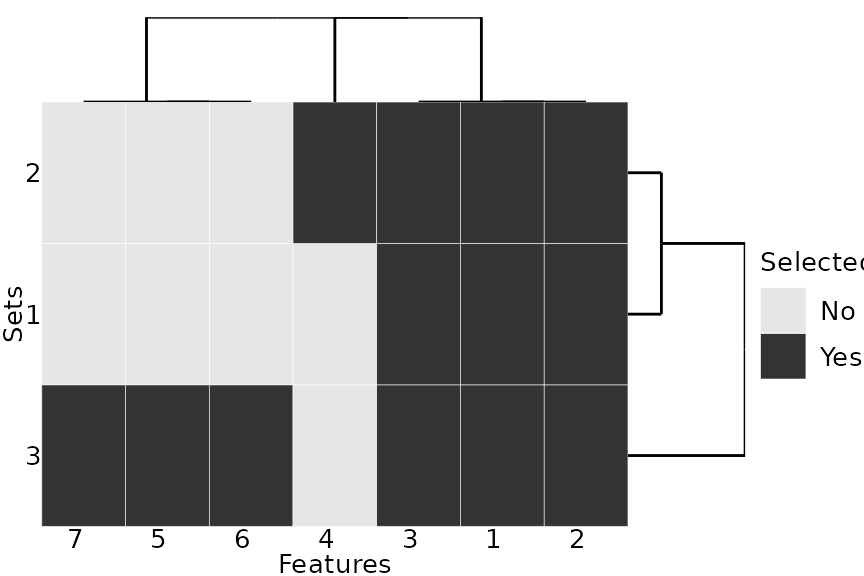
Example: Feature Selection
In this example, we will analyze the stability of the feature
selection of regression trees on the BostonHousing2 data
set from the mlbench
package.
library(rpart) # for classification trees
data("BostonHousing2", package = "mlbench")

# remove feature that is a version of the target variable
dataset = subset(BostonHousing2, select = -cmedv)
We write a small function which subsamples the
BostonHousing2 data frame to ratio percent of
the observations, fits a regression tree and then returns the used
features as character vector:
fit_tree = function(target = "medv", data = dataset, ratio = 0.67, cp = 0.01) {
    n = nrow(data)
    i = sample(n, n * ratio)
    formula = as.formula(paste(target,  "~ ."))
    model = rpart::rpart(formula = formula, data = data, subset = i,
      control = rpart.control(maxsurrogate = 0, cp = cp))
    names(model$variable.importance)
}

set.seed(1)
fit_tree()
## [1] "rm" "lstat" "town" "crim"We repeat this step 30 times, resulting in a list of character vectors of selected features:
A quick analysis of the list reveals that three features are selected in all repetitions while six other features are only selected in some of the repetitions:
# Selected in each repetition:
Reduce(intersect, selected_features)
## [1] "rm" "lstat" "town"
# Sorted selection frequency across all 30 repetitions:
sort(table(unlist(selected_features)), decreasing = TRUE)
##
## lstat rm town crim dis age lon ptratio tract
## 30 30 30 6 4 3 2 2 1The selection frequency can be visualized with the
plotFeatures() function:
plotFeatures(selected_features)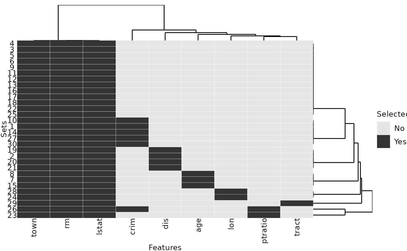
To finally express the selection frequencies with one number, e.g. to compare the stability of regression trees to the stability of a different modeling approach, any of the implemented stability measures can be calculated:
stabilityJaccard(selected_features)## [1] 0.7622989We consider a second parametrization of regression trees and observe that this parametrization provides a more stable feature selection than the default parametrization: the value of the Jaccard stability measure is higher here:
set.seed(1)
selected_features2 = replicate(30, fit_tree(cp = 0.02), simplify = FALSE)
stabilityJaccard(selected_features2)
## [1] 0.9089655
plotFeatures(selected_features2)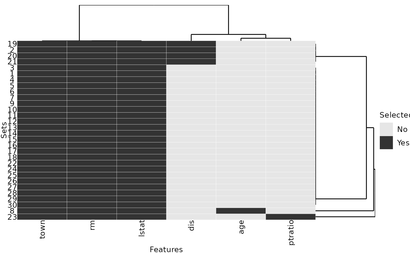
Now, we consider a different regression problem, for which there are highly correlated features. Again, we repeatedly select features using regression trees:
dataset2 = subset(BostonHousing2, select = -town)
dataset2$chas = as.numeric(dataset2$chas)

set.seed(1)
selected_features3 = replicate(30, fit_tree(target = "rm", data = dataset2, cp = 0.075),
  simplify = FALSE)
We choose to assess the similarities between the features with absolute Pearson correlations, but other similarity measures could be used as well. The similarity values of the selected features show that the two features medv and cmedv are almost perfectly correlated:
# similarity matrix
sim.mat = abs(cor(subset(dataset2, select = -rm)))

sel.feats = unique(unlist(selected_features3))
sim.mat[sel.feats, sel.feats]
## medv dis cmedv lstat
## medv 1.0000000 0.2499287 0.9984759 0.7376627
## dis 0.2499287 1.0000000 0.2493148 0.4969958
## cmedv 0.9984759 0.2493148 1.0000000 0.7408360
## lstat 0.7376627 0.4969958 0.7408360 1.0000000Also, each of the 30 feature sets includes either medv or cmedv:
plotFeatures(selected_features3, sim.mat = sim.mat)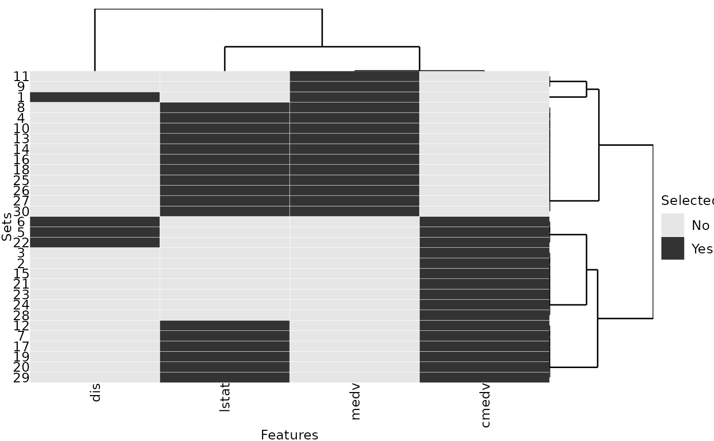
When evaluating the feature selection stability, we want that the
choice of medv instead of cmedv or vice versa is not
seen as a lack of stability, because they contain almost the same
information. Therefore, we use one of the adjusted stability
measures, see listStabilityMeasures() in Section
Usage.
stabilityIntersectionCount(selected_features3, sim.mat = sim.mat, N = 100)## [1] 0.7677557The effect of the feature similarities for stability assessment can be quantified by considering the identity matrix as similarity matrix and thereby neglecting all similarities. Without taking into account the feature similarities, the stability value is much lower:
no.sim.mat = diag(nrow(sim.mat))
colnames(no.sim.mat) = row.names(no.sim.mat) = colnames(sim.mat)
stabilityIntersectionCount(selected_features3, sim.mat = no.sim.mat)
## [1] 0.4168795Example: Clustering
As a second example, we analyze the stability of the clusters resulting from k-means clustering.
set.seed(1)

# select a subset of instances for visualization purposes
inds = sample(nrow(dataset2), 50)
dataset.cluster = dataset2[inds, ]

# run k-means clustering with k = 3 30 times
km = replicate(30, kmeans(dataset.cluster, centers = 3), simplify = FALSE)

# change cluster names for comparability
best = which.min(sapply(km, function(x) x$tot.withinss))
best.centers = km[[best]]$centers
km.clusters = lapply(km, function(kmi) {
  dst = as.matrix(dist(rbind(best.centers, kmi$centers)))[4:6, 1:3]
  rownames(dst) = colnames(dst) = 1:3
  # greedy choice of best matches of clusters
  new.cluster.names = numeric(3)
  while(nrow(dst) > 0) {
    min.dst = which.min(dst)
    row = (min.dst - 1) %% nrow(dst) + 1
    row.o = as.numeric(rownames(dst)[row])
    col = ceiling(min.dst / nrow(dst))
    col.o = as.numeric(colnames(dst)[col])
    new.cluster.names[row.o] = col.o
    dst = dst[-row, -col, drop = FALSE]
  }
  new.cluster.names[kmi$cluster]
})

# for each cluster, create a list containing the instances
# belonging to this cluster over the 30 repetitions
clusters = lapply(1:3, function(i) {
  lapply(km.clusters, function(kmc) {
    which(kmc == i)
  })
})
For each cluster, we evaluate the stability of the instances assigned to this cluster:
stab.cl = sapply(clusters, stabilityJaccard)
stab.cl
## [1] 0.8488756 0.8037725 0.5485411We average these stability values with a weighted mean based on the average cluster sizes:
## [1] 0.7730162